2. Molecular Parameters and Energy Level Formulation

In spite of the fact that triatomic molecules are the simplest polyatomic species, a thorough discussion of the theoretical background of their rotational spectra and energy level interactions would entail an extensive text in itself, and would require repetition of many excellent treatments readily available. Thus, the discussion which follows deals with the most common cases which will provide the user with the essential definition of quantum numbers, molecular parameters and basic relations employed in the analysis of rotational spectra. For the reader interested in a more detailed description of polyatomic rotational spectral measurements and analysis, we refer to texts on this subject by Townes and Schawlow [3], Gordy and Cook [4], Wollrab [5] and Kroto [6] which have both detailed and excellent discussions of all facets of rotational spectra. The spectroscopic notation employed follows, as closely as possible, the recommendations of the Joint Commission for Spectroscopy of the International Astronomical Union and the International Union of Pure and Applied Physics [7].

a. Linear Triatomic Molecules

(eq1)

The selection rules for rotational transitions of a linear polyatomic molecule are ΔJ = 0, ±1, and Δℓ=0, ±1, where J is the total angular momentum quantum number excluding nuclear spin and ℓ is the vibrational angular momentum quantum number which arises in degenerate bending vibrational states.

Since molecules are not rigid, the effects of molecular vibrations and centrifugal distortion must be included in the model in order to accurately fit the observed rotational spectra. The rotational energy levels are represented as:

(eq2)

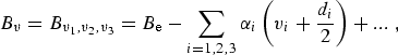
where B_υ is the rotational constant for the υ^th vibrational state, and D_υ and H_υ are the centrifugal distortion constants. The rotational constant can be expressed in terms of its equilibrium value, B_e, and rotation-vibration interaction constants, α_i, as:

(eq3)

neglecting higher order terms. Within this level of approximation rotational transitions from lower state J″ to upper state J′ are expressed:

(eq4)

The treatment of rotational transitions in excited vibrational states requires additional terms to account for the rotation�vibration interactions. The symmetry species of excited vibrational states are designated as Σ, Π, Δ, etc., when ℓ = 0, ± 1, ± 2, etc., respectively. One of the most common rotation-vibration interactions is ℓ-type doubling in Π states. In this case each J → J + 1 transition has two components which are indicated as L (lower) and U (upper) components in the tables which follow. The doublet separation is represented as: q_υ(υ + 1)(J + 1). In addition ΔJ = 0 transitions are observable with the frequency expressed as: ν = (q_υ/2)(υ + 1)J(J + 1). These transitions are also included in the spectral tables. Other rotation-vibration interactions, such as Fermi resonance, often must be included for particular measurements. Since the level of approximation and method of analysis is dependent on the extent and quality of the spectral measurements available, the user should refer to the literature references cited in the tables for details concerning the analysis. For more general treatments of ℓ-type doubling and resonance interactions see the texts mentioned earlier [3-6] or the review by D.R. Lide [8].

Hyperfine structure is observable in a majority of the linear molecules tabulated here. Hyperfine structure stems from nuclear electric quadrupole interaction with the electric field gradient at the nucleus, magnetic interaction of nuclear spin with the field produced by molecular rotation, and interaction between the two nuclear spins. Basically, only the nuclear quadrupole and spin-rotation effects have been observed in microwave rotational spectra, while all of the hyperfine structure interactions of a number of triatomics have been determined from molecular beam electric resonance studies. Since the treatment of these effects can become quite complex and often handled individually for each case, the reader is referred to the literature cited for particular formulations. Rather detailed general treatments of hyperfine structure in molecular spectra can be found in references [3-6] as well as in references to laboratory studies of individual species.

The most common case observed is that for triatomic molecules which contain one nucleus with nuclear spin, I ≥ 1. In this case, the nuclear electric quadrupole and spin�rotation interactions from first order perturbation theory add to the rotational energy via:

(eq5)

where f(I,J,F) is Casimir's function which is tabulated in Appendix I of reference [3] and Appendix IV of reference [4]. Here F is the total angular momentum quantum number, where F = J + I, J + I - 1, ... |J = I|. The additional selection rule for transitions between rotational levels split by hyperfine structure is ΔF = 0, �1.

When the molecule exhibits hyperfine splittings from more than one nucleus, an exact matrix diagonalization of the Hamiltonian is usually required. Although the vector coupling model to be employed varies according to the magnitude of the interaction between J, I₁, and I₂, the typical case is to label the nucleus causing the largest interaction as I₁, thus

(eq6a)

and

(eq6b)

For detailed discussions of the coupling schemes and matrix elements for multiple nuclear electric quadrupole interactions see [4] and [5].

b. Non-Linear Triatomic Molecules

The rotational energy levels are characterized by the three quantum numbers J_K-1,K+1 in the King-Hainer-Cross notation. Here, since S=0, J is used rather than N for the rotational angular momentum. When S≠0 we will use N_K-1,K+1 to designate the rotational state and J for rotation plus electron spin and orbital angular momenta. The K_-1 subscript is the K value in the limiting case of prolate symmetric-top and K₊₁ corresponds to the limiting case for an oblate symmetric-top. Ray's asymmetry parameter, κ, is often used to characterize the degree of asymmetry:

(eq7)

When A ≈ B, κ approaches +1 for the oblate case and when B ≈ C, κ approaches -1 for the prolate case.

1) Selection Rules

(eq8a)

and b-type transitions follow the selection rules

(eq8b)

When a triatomic molecule has a symmetry axis, for example in the XY₂ molecules, only b-type transitions can occur. In these cases one must also examine the nuclear spin statistics which influence both the selection rules and population of the rotational levels.

2) Rotational and Centrifugal Distortion Constants

(eq9)

where α,β = a,b, or c. For a planar molecule the following planarity relations reduce the six linear combinations of distortion constants to four and provide the determinable parameters shown in column 1 of table 2.1:

(eq10)

(eq11)

(eq12)

(eq13)

For non-planar molecules Dreizler et al. [11,12] found the Kivelson-Wilson distortion constants were indeterminant. Watson [13,14] introduced a new relationship which allows the Kivelson-Wilson Hamiltonian to be expressed in terms of five independent centrifugal distortion coefficients, or linear combination of taus, which eliminates the indeterminancy noted by Dreizler et al. Much of the recent analysis of rotational spectra follow Watson's reformulation [15,16] in the form of a reduced Hamiltonian which simplified the computation of the energy levels.

Table 2.1. Determinable Rotational and Centrifugal Distortion Constants (P ⁴) Employed by Various Workers ^a

Kivelson-Wilson parameters for planar molecules	Kirchhoff parameters (following Watson [15])	Watson parameters [16]
A′	A″ = A′ - 1/2τbbcc′
B′	B″ = B′ - 1/2τaacc′
C′	C″ = C′ - 1/2τaabb′
τaaaa	τaaaa	ΔJ
τbbbb	τbbbb	ΔJK
τabab	τcccc	ΔK
τaabb	τ1 = τaabb′ + τbbcc′ + τccaa′	δJ
	τ2 = (A′ / S) τbbcc′ + (B′ / S) τaacc′ + (C′ / S) τaabb′	δK
	τ3 = [S / (B′ - A′)]τaabb′ + [S / (A′ - C′)]τaacc′ + [S / (C′ - B′)]τbbcc′ where S = A′ + B′ + C′

^aFor conversion between the various sets of parameters see references [4], [9], [10], and [17].

Since there is not a unique unitary transformation which allows the nine Kivelson-Wilson parameters to be reduced to eight determinable parameters, several variations of the Watson reduced Hamiltonians are commonly employed in practice. The two most often employed result in the determinable parameters listed in columns 2 and 3 of table 2.1. In reanalyzing the microwave spectra of triatomic molecules, Kirchhoff's [10] formulation has been used and the planarity conditions have been invoked in the spectral fitting process to fix τ₃. See reference [10] for additional details. The second commonly used formulation is described in detail by Gordy and Cook [4]. Yamada and Winnewisser [17] have examined the effects of employing different reductions for the three King, Hairier and Cross axis representations I^r, II^r, and III^r [18]. They provide a useful set of relations between the spectroscopic constants determined in the various reduction procedures and discuss the implications of the τ defect when employing the planarity conditions. When the spectral data requires a higher order Hamiltonian, such as inclusion of P⁶ terms, generally the first-order perturbation treatment suggested by Watson [16] has been used. For some light molecules such as H₂O and H₂S even higher order terms were needed. See Gordy and Cook [4] or the sources of the spectroscopic constants quoted in the tables on these species.

c. Molecules with Doublet Electronic Ground States

These interactions and the Hamiltonian for such molecules are discussed by Lin [19], Van Vleck [20], Curl and Kinsey [21] and others. Curl and Kinsey [21] have summarized the spectroscopic constant notation employed in the various formulations and developed an alternate method which can be applied to the triatomic species. Since none of these species have been reanalyzed in the present work, the notation employed in the publications cited is followed in the present tables of spectroscopic constants.