Auto, Cross Correlation Menu

The 'Correlation' menu displays the auto and cross correlation interface, which allows the user to perform the correlation analysis on a profile.

To perform the autocorrelation analysis:

1. On the right menu, select the type of a profile, such as total profile, primary profile, waviness, or roughness.
2. Select calculation method (use FFT or Time domain to calculate Autocorrelation)
3. Enter lag length into a text field below calculation method.
4. Click on the 'Calculate' button to perform the analysis.


To perform the cross correlation analysis on profile 1 and 2  (profile 1 and 2 must have the same spacing in x-direction):

1. On the right menu, select type of a profile, such as total profile, primary profile, waviness, or roughness at profile 1.
2. For profile 2, click on the 'Browse' button, which displays a File Open dialog. The user then needs to change the sdf data file format from the 'Files of type' combo box for file selection.
3. Select calculation method (use Spatial Domain or Spatial Frequency Domain to calculate Auto-corellation)
4. Enter lag length into a text field below the calculation method.
5. Click on 'Calculate' button to perform the analysis.


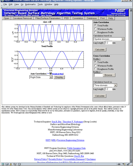
The result shows two plots. The first one shows the profile that was selected for correlation analysis. The second one shows the correlation curve. The correlation curve can be viewed on the right side or both right and left sides. This can be done by selecting the drop down menu bellow the correlation curve, and click on 'Display" button.


To download analysis data:
1. Click on the floppy disk icon and the Save dialog will display. It will ask the user where a zip file will be saved.
2. When the zip file is opened, the user will see data files in XML, DTD, and SDF data format.