 |
(eq 1) |
The selection rules for rotational transitions of a linear polyatomic molecule are ΔJ = 0, ±1, and Δℓ = 0, ±1; where J is the total angular momentum quantum number excluding nuclear spin and ℓ is the vibrational angular momentum quantum number which arises in degenerate bending vibrational states.
Since molecules are not rigid, the effects of molecular vibrations and centrifugal distortion must be included in the model in order to accurately fit the observed rotational spectra. The rotational energy levels are represented as:
 |
(eq 2) |
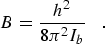
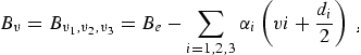
where Bv, is the rotational constant for the nth vibrational state, and Dv, and Hv, are the centrifugal distortion constants. The rotational constant can be expressed in terms of its equilibrium value, Be, and rotation-vibration interaction constants, αi, as
 |
(eq 3) |
neglecting higher order terms. Within this level of approximation the frequencies of rotational transitions from lower state J′′ to upper state J′ = J′′ + 1 are expressed:
 |
(eq 4) |
The treatment of rotational transitions in excited vibrational states requires additional terms to account for the rotation-vibrational interactions. The symmetry species of excited vibrational states are designed as Σ, Π, Δ, etc., when ℓ = 0, ±1, ±2, etc., respectively. One of the most common rotation-vibration interactions is ℓ-type doubling in Π states. In this case each J→J + 1 transition has two components which are indicated as L (lower) and U (upper) components in the tables which follow. The doublet separation is represented as: qv(v + 1)(J + 1). In addition ΔJ = 0 transitions are observable with the frequency expressed as: v = (qv/2)(v+1)J(J+1). These transitions are also included in the spectral tables. Other rotation-vibration interactions, such as Fermi resonance, often must be included for particular measurements. Since the level of approximation and method of analysis is dependent on the extent and quality of the spectral measurements available, the user should refer to the literature references cited in the tables for details concerning the analysis. For more general treatments of ℓ-type doubling and resonance interactions see the texts mentioned earlier [4 to 7] or the review by D.R. Lide [9].
 |
(eq 5) |
including the first order (P4) centrifugal distortion terms. The selection rules are ΔJ = 0, ±1, ΔK = 0. The frequency for a J + 1 ← J and K ← K rotational transition is
 |
(eq 6) |
which includes the P6 centrifugal distortion terms.
As in the case of linear molecules, vibrationally excited states can exhibit ℓ-type doubling which arises from the degenerate bending vibrational modes. Formulas for the rotational levels are given in the references cited in the molecular parameter tables here, e.g., propyne references, as well as in some of the text books referenced here [5] to [7].
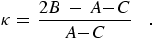
The rotational energy levels are characterized by the three quantum numbers JK-1,K+1 in the King-Hainer-Cross notation. Here, since S = 0, J is used rather than N for the rotational angular momentum. When S ≠ 0 we will use NK-1,K+1 to designate the rotational state and J for rotation plus electron spin and orbital angular momenta. The K-1 subscript is the K value in the limiting case of prolate symmetric-top and K+1 corresponds to the limiting case for an oblate symmetric-top. Ray's asymmetry parameter, κ, is often used to characterize the degree of asymmetry:
 |
(eq 7) |
When A ≈ B, κ approaches +1 for the oblate case and when B ≈ C, κ approaches -1 for the prolate case.
(1) Selection Rules
In general an asymmetric rotor can exhibit three types of pure rotational transitions if the molecule has nonzero components of the electric dipole moment in the direction of the a, b, and c principal axes. For an asymmetric rotor the selection rules for a-type transitions are:
 |
(eq 8) |
for b-type transitions:
 |
(eq 9) |
for c-type transitions:
 |
(eq 10) |
When a molecule has a symmetry axis one must also examine the nuclear spin statistics that influence both the selection rules and the populations of the rotational levels.
(2) Rotational and Centrifugal Distortion Constants
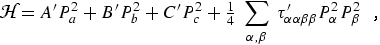
Until approximately 1970 the Kivelson and Wilson [10] formulation of the Hamiltonian for a non-rigid asymmetric rotor was widely employed in analyzing rotational spectra. With the parameter notation employed by Kirchhoff [11] the Kivelson-Wilson Hamiltonian is:
 |
(eq 11) |
where α,β = a, b, or c. For a planar molecule the following planarity relations reduce the six linear combinations of distortion constants to four and provide the determinable parameters shown in column 1 of Table 2.1:
 |
(eq 12a) |
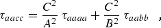 |
(eq 12b) |
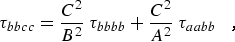 |
(eq 12c) |
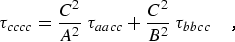 |
(eq 12d) |
For non-planar molecules Dreizler et al. [12,13] found that the Kivelson-Wilson distortion constants were indeterminant. Watson [14,15] introduced a new relationship which allows the Kivelson-Wilson Hamiltonian to be expressed in terms of five independent centrifugal distortion coefficients, or linear combinations of taus, which eliminates the indeterminancy noted by Dreizler et al. Much of the recent analysis of rotational spectra follows Watson's reformulation [16,17] in the form of a reduced Hamiltonian which simplified the computation of the energy levels.
Since there is not a unique unitary transformation which allows the nine Kivelson-Wilson parameters to be reduced to eight determinable parameters, several variations of the Watson reduced Hamiltonian are commonly employed in practice. The two most often employed result in the determinable parameters listed in columns 2 and 3 of Table 2.1. In reanalyzing the microwave spectra here both Kirchhoff's [11] formulation has been used as well as Watson's A-reduction [17]. See reference [11] for additional details. The second commonly used formulation is described in detail by Gordy and Cook [5]. Yamada and Winnewisser [18] have examined the effects of employing different reductions for the three King, Hainer and Cross axis representations Ir, IIr, and IIIr [19]. They provide a useful set of relations between the spectroscopic constants determined in the various reduction procedures and discuss the implications of the τ defect when employing the planarity conditions. When the spectral data require a higher order Hamiltonian, such as inclusion of P6 terms, generally the first-order perturbation treatment suggested by Watson [17] has been used.
| a) | N + S = J; J + I = F | ||
| b) | S + I = G; G + N = F | ||
| c) | N + I = E; E + S = F | . |
These interactions and the Hamiltonian for such molecules are discussed by Lin [20], Van Vleck [21], Curl and Kinsey [22] and others. Curl and Kinsey [22] have summarized the spectroscopic constant notation employed in the various formulations and developed an alternate method which can be applied to the hydrocarbon species. Since none of these species have been reanalyzed in the present work, the notation employed in the publications cited is followed in the present tables of spectroscopic constants.
|
||||